

Introduction of the project
Today we will make a coding project on House Price Prediction Using Python. This machine learning model helps us to predict the price of a house on the basis of features like BHK, area, locality, etc. This model acts as a helping hand to the people engaged in the real estate industry. We have created this model through the dataset of Bangalore city, where the model predicts the price of a property on the basis of various features of the house in Bangalore.
Objectives
- The objective of building this machine learning model is to help clients in the real estate industry. This will help the people looking for a place to live to select the best property for living based on their own specifications and utility.
- To give the estimated price of a house according to the features so that users can get the best-fit property for their living purpose with their needs of the area, locality and rates accordingly.
- To act as an interface between the real estate industry and specific clients associated with it.
Requirements
1. Python Libraries
- Pandas
- NumPy
- Matplotlib
2. Jupyter Notebook or Google Colab
3. Dataset
Source Code
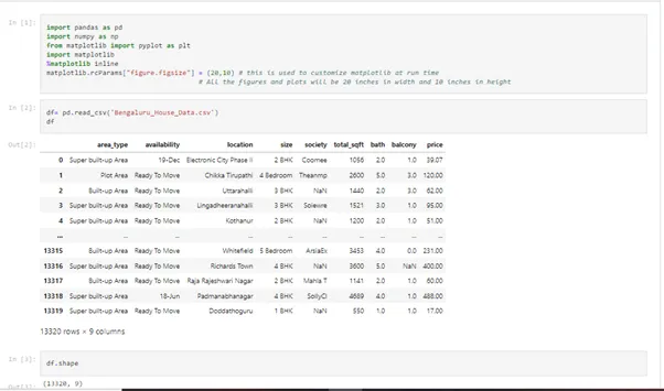
import pandas as pd
import numpy as np
from matplotlib import pyplot as plt
import matplotlib
%matplotlib inline
matplotlib.rcParams["figure.figsize"] = (20,10) # this is used to customize matplotlib at run time
# All the figures and plots will be 20 inches in width and 10 inches in height
df= pd.read_csv('Bengaluru_House_Data.csv')
df
df.shape
df['area_type'].value_counts() # This will keep a count on total how many areas are presen
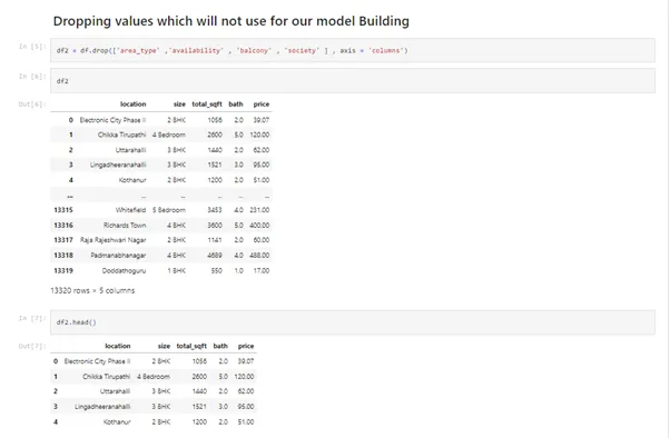
df2 = df.drop(['area_type' ,'availability' , 'balcony' , 'society' ] , axis = 'columns')
df2
df2.head()
df2.isnull() # checking if any missing value is present or not
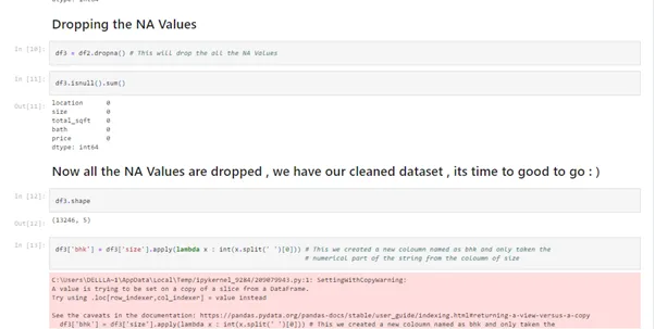
df2.isnull().sum() # This shows the NA values
df3 = df2.dropna() # This will drop the all the NA Values
df3.isnull().sum()
df3.shape
df3['bhk'] = df3['size'].apply(lambda x : int(x.split(' ')[0])) # This we created a new coloumn named as bhk and only taken the
# numerical part of the str
df3.head()
df3['bhk'].unique()
df3[df3.bhk>20]
# exploring total_sqft
df3['total_sqft'].unique()
df3['location'].value_counts
def is_float(x):
try:
float(x)
except:
return False
return True
df3[~df3['total_sqft'].apply(is_float)]
def convert_sqft_to_num(x):
tokens = x.split('-')
if len(tokens) == 2:
return (float(tokens[0])+float(tokens[1]))/2
try:
return float(x)
except:
return None
df4 = df3.copy() # creating a new data frame
df4['total_sqft'] = df4['total_sqft'].apply(convert_sqft_to_num) # applying the function within our coloumn of our new data frame
df4.head()
df4.loc[30]
df4.head()
df5 = df4.copy()
# now its time to create a coloumn of price per square feet as its important for real estate
df5['price_per_sqft'] = df5['price']*100000/df5['total_sqft']
df5.head()
df5.location.unique()
len(df5.location.unique())
df5.location = df5.location.apply(lambda x : x.strip()) # this is to remove the irregularities in location text data
# checking the number of data rows of different locations
location_stats = df5.groupby('location')['location'].agg('count')
location_stats
# sorting in descending order
location_stats = df5.groupby('location')['location'].agg('count').sort_values(ascending = False)
location_stats
len(location_stats[location_stats<=10]) # checking the number of locations with less than or equal to 10 data points
location_stats_less_than_ten = location_stats[location_stats<=10]
location_stats_less_than_ten
df5.location = df5.location.apply(lambda x : 'other' if x in location_stats_less_than_ten else x)
len(df5.location.unique())
df5.head(10)
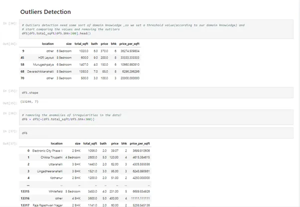
# Outliers detection need some sort of domain knowledge ,so we set a threshold value(according to our domain knowledge) and
# start comparing the values and removing the outliers
df5[df5.total_sqft/df5.bhk<300].head()
df5.shape
# removing the anamolies of irregularities in the data!
df6 = df5[~(df5.total_sqft/df5.bhk<300)]
df6
df5.shape
df6.shape
df6.price_per_sqft.describe()
# setting a threshold and considering only that values which will greater than (m-st) and smaller than (m+st)
def remove_pps_outliers(df):
df_out = pd.DataFrame()
for key, subdf in df.groupby('location'):
m = np.mean(subdf.price_per_sqft)
st = np.std(subdf.price_per_sqft)
reduced_df = subdf[(subdf.price_per_sqft>(m-st)) & (subdf.price_per_sqft<=(m+st))]
df_out = pd.concat([df_out,reduced_df],ignore_index=True)
return df_out
df7 = remove_pps_outliers(df6)
df7.shape
df7
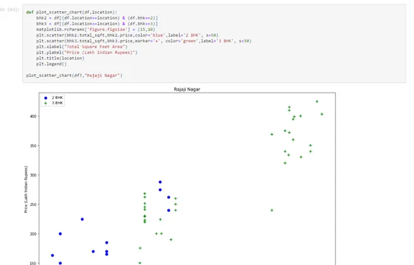
def plot_scatter_chart(df,location):
bhk2 = df[(df.location==location) & (df.bhk==2)]
bhk3 = df[(df.location==location) & (df.bhk==3)]
matplotlib.rcParams['figure.figsize'] = (15,10)
plt.scatter(bhk2.total_sqft,bhk2.price,color='blue',label='2 BHK', s=50)
plt.scatter(bhk3.total_sqft,bhk3.price,marker='+', color='green',label='3 BHK', s=50)
plt.xlabel("Total Square Feet Area")
plt.ylabel("Price (Lakh Indian Rupees)")
plt.title(location)
plt.legend()
plot_scatter_chart(df7,"Rajaji Nagar")
df7.head(5)
# now removing the outliers
def remove_bhk_outliers(df):
exclude_indices = np.array([])
for location, location_df in df.groupby('location'):
bhk_stats = {}
for bhk, bhk_df in location_df.groupby('bhk'):
bhk_stats[bhk] = {
'mean': np.mean(bhk_df.price_per_sqft),
'std': np.std(bhk_df.price_per_sqft),
'count': bhk_df.shape[0]
}
for bhk, bhk_df in location_df.groupby('bhk'):
stats = bhk_stats.get(bhk-1)
if stats and stats['count']>5:
exclude_indices = np.append(exclude_indices, bhk_df[bhk_df.price_per_sqft<(stats['mean'])].index.values)
return df.drop(exclude_indices,axis='index')
df8 = remove_bhk_outliers(df7)
# df8 = df7.copy()
df8.shape
plot_scatter_chart(df8 , 'Rajaji Nagar') # plotting the difference after removing the outlier
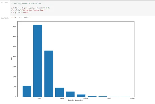
# Sort off normal distribution
plt.hist(df8.price_per_sqft,rwidth=0.8)
plt.xlabel("Price Per Square Feet")
plt.ylabel("Count")
df8.bath.unique()
df8[df8.bath>10]
plt.hist(df8.bath , rwidth = 0.8)
plt.xlabel("Number Of Bathrooms")
plt.ylabel("Counts")
df8[df8.bath>df8.bhk+2]
df9 = df8[df8.bath<df8.bhk+2]
df9.shape # we have only considered the data in which bathrooms are less than the bhk and setted in a new data frame
# Now dropping all the necessary coloumns for training and testing process
df10 = df9.drop(['size' , 'price_per_sqft'] , axis = 'columns')
df10.head(5)
dummies = pd.get_dummies(df10.location) # as location is the text data so we need to convert it into numerical so that our model
# could handle the data
dummies.head(3)
# this is one hot encoding
df11 = pd.concat([df10 , dummies.drop('other' , axis = 'columns') ] , axis = 'columns')
df11.head(5)
df12 = df11.drop('location' , axis = 'columns')
df12
df12.shape
X = df12.drop('price' , axis = 'columns')
X.head()
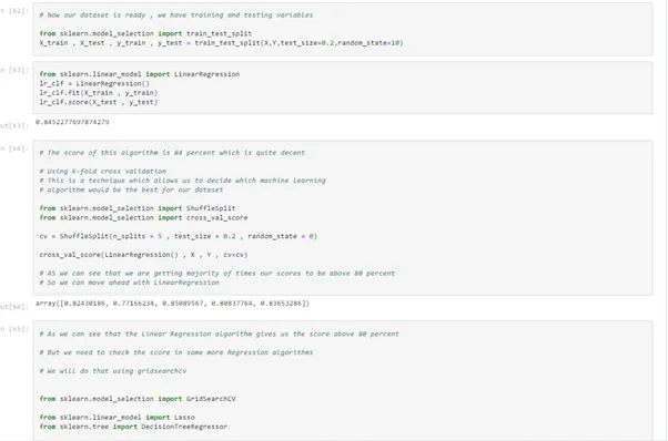
# Now our dataset is ready , we have training and testing variables
from sklearn.model_selection import train_test_split
X_train , X_test , y_train , y_test = train_test_split(X,Y,test_size=0.2,random_state=10)
from sklearn.linear_model import LinearRegression
lr_clf = LinearRegression()
lr_clf.fit(X_train , y_train)
lr_clf.score(X_test , y_test)
# The score of this algorithm is 84 percent which is quite decent
# Using K-fold cross validation
# This is a technique which allows us to decide which machine learning
# algorithm would be the best for our dataset
from sklearn.model_selection import ShuffleSplit
from sklearn.model_selection import cross_val_score
cv = ShuffleSplit(n_splits = 5 , test_size = 0.2 , random_state = 0)
cross_val_score(LinearRegression() , X , Y , cv=cv)
# AS we can see that we are getting majority of times our scores to be above 80 percent
# So we can move ahead with LinearRegression
# As we can see that the Linear Regression algorithm gives us the score above 80 percent
# But we need to check the score in some more Regression algorithms
# We will do that using gridsearchcv
from sklearn.model_selection import GridSearchCV
from sklearn.linear_model import Lasso
from sklearn.tree import DecisionTreeRegressor
def find_best_model_using_gridsearchcv(X,y):
algos = {
'linear_regression' : {
'model': LinearRegression(),
'params': {
'normalize': [True, False]
}
},
'lasso': {
'model': Lasso(),
'params': {
'alpha': [1,2],
'selection': ['random', 'cyclic']
}
},
'decision_tree': {
'model': DecisionTreeRegressor(),
'params': {
'criterion' : ['mse','friedman_mse'],
'splitter': ['best','random']
}
}
}
scores = []
cv = ShuffleSplit(n_splits=5, test_size=0.2, random_state=0)
for algo_name, config in algos.items():
gs = GridSearchCV(config['model'], config['params'], cv=cv, return_train_score=False)
gs.fit(X,y)
scores.append({
'model': algo_name,
'best_score': gs.best_score_,
'best_params': gs.best_params_
})
return pd.DataFrame(scores,columns=['model','best_score','best_params'])
find_best_model_using_gridsearchcv(X,Y)
X.columns
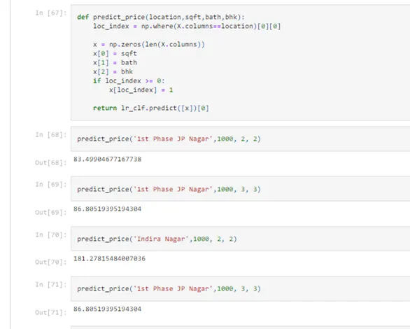
def predict_price(location,sqft,bath,bhk):
loc_index = np.where(X.columns==location)[0][0]
x = np.zeros(len(X.columns))
x[0] = sqft
x[1] = bath
x[2] = bhk
if loc_index >= 0:
x[loc_index] = 1
return lr_clf.predict([x])[0]
predict_price('1st Phase JP Nagar',1000, 2, 2)
Explanation of the Code
1. Initially, we imported all the necessary libraries that will be required for this prediction model and loaded our dataset for analysis.
2. After importing the necessary python libraries, we perform a cleaning of the dataset.
3. Checking the null values and accordingly dropping them to clean the dataset further.
4. Once the dataset has been cleaned, then we start detecting the outliers.
5. Now, we have used the matplotlib library to visualize our dataset.
6. Next is the Train Test Split phase and using the K-fold cross-validation to select the best algorithms.
Output
Finally, the house price prediction using python model is ready with a predict function which will predict the price of a house on the basis of given parameters passed in the predict function accordingly.
Conclusion
This machine learning model of House Price Prediction Using Python helps the clients to select the best property according to their own utility and demand as this model predicts the price of the house on the basis of features like BHK, area in square feet, locality, etc. This coding project can serve as a helping hand in the real estate industry and can make the process of buying a house in a specific area accessible.